OpenCV 基本操作

1. 图像读取

   import cv2
   img_uint = cv2.imread(path)
   
   img_uint = cv2.cvtColor(img, cv2.COLOR_BGR2RGB)
   img = img_uint / 255.
   

   • cv2 默认读取 BGR, uint8(0 - 255) => (h, w, c)

2. 图像显示

   from matplotlib import pyplot as plt
   _, ax = plt.subplots(1, 2, figsize=(10, 5))
   # ----------
   # plt.figure(figsize=(10, 5))
   # ax = plt.gca()
   # ----------
   # plt.subplot(1, 2, 1)
   # ax = plt.gca()
   ax.imshow(img)
   ax.axis('off')
   

3. 图像变换

   • Translation
     在齐次坐标 \begin{bmatrix}x \\ y \\ 1\end{bmatrix} 下，存在平移矩阵 M=\begin{bmatrix}1 & 0 & c_x \\ 0 & 1 & c_y\end{bmatrix}

     M = np.float32([[1, 0, 100],
                     [0, 1, 50]])
     rows, cols = img.shape[:2]
     res = cv2.warpAffine(img, M, (rows, cols))
     

     padding 部分填充为 (0, 0, 0)

   • Rotation
     这里就不自己算旋转矩阵了，通过cv2.getRotationMatrix2D((center_x, center_y), angle, scale)得到对应的变换矩阵

     M = cv2.getRotationMatrix2D((h/2, w/2), 45, 1)
     res = cv2.warpAffine(img, M, (h, w))
     

   • Scaling

     h, w = img.shape[:2]
     res = cv2.resize(img, None, fx=2, fy=2, interpolation=cv2.INTER_CUBIC)
     # res = cv2.resize(img, (2*h, 2*w), interpolation=cv2.INTER_CUBIC)
     

     插值方法包括
     - cv2.INTER_NEAREST
     - cv2.INTER_CUBIC 三次样条
     - cv2.INTER_LINEAR
     - cv2.INTER_AREA 自动选择方案

   • 仿射 Affine

     pts1 = np.float32([[50, 50],
                        [200, 50],
                        [50, 200]])
     pts2 = np.float32([[10, 100],
                        [200, 50],
                        [100, 250]])
     M = cv2.getAffineTransform(pts1, pts2)
     res = cv2.warpAffine(img, M, (h, w))
     

   • 透射 Perspective

     M = cv2.getPerspectiveTransform(pts1, pts2)
     

     透射变换需要给出 4 个定位点

色彩分析

1. 灰度变换

   img_linear = 0.5 * img + 0.5
   img_power_light = np.power(img, 0.5)
   img_power_dark = np.power(img, 2)
   img_log = np.log(img + 1) / np.log(2)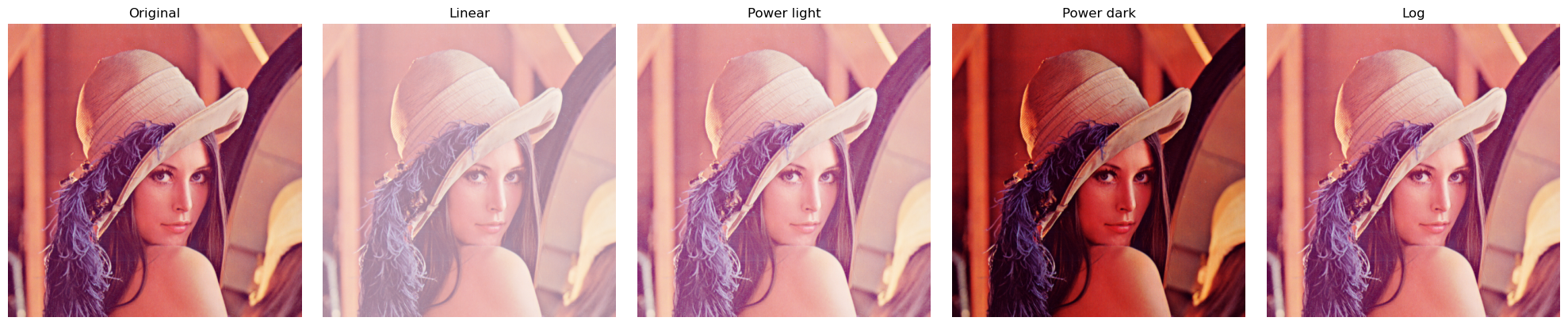
   

   

2. 通道分离

   r, g, b = cv2.split(img_uint)
   

3. 直方图提取

   hist_r = cv2.calcHist([r], [0], None, [256], [0, 256])
   

   Params:

   • image: 可以是一个 list of images，需要保持相同的 dtype 和 size

   • channels: 这里是单通道的

   • mask (optional)

   • histSize

   • ranges

   直方图可以用来做什么？一个例子
   来自 https://zhuanlan.zhihu.com/p/24507450
   
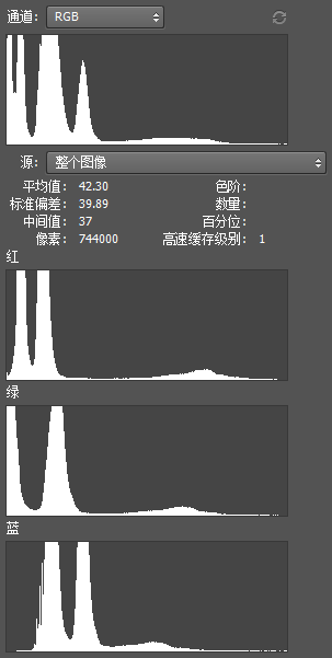
   我们来观察这张直方图

   1. 蓝色通道左侧是 0，表示没有一个像素 B 值是 0，而绿色和红色左侧都有很多凸起，表示整张图片强烈地呈现出蓝色
   2. 观察红绿蓝都有一个小山丘在右侧，这代表一小部分像素 rgb 值较大，所以偏向白色，是高光部分；高光部分红色凸起最靠右，这是因为原图高光是人脸和衣服，而人脸和衣服都满足 r>g>b

4. 直方图均衡化

   img_uint_gray = cv2.cvtColor(img_uint, cv2.COLOR_RGB2GRAY)
   img_uint_equalized_gray = cv2.equalizeHist(img_unit_gray)
   

   • 这使得每个亮度区间内的像素数量都相同 => 增强对比度
   • 输入必须是单通道(GRAY) + uint8