这是 2025 春 计算机视觉导论的笔记
Todo:
- 内容杂乱无章,十分愚蠢,或许未来会润色语言使它便于阅读
Images as Functions
Image as a function
我们把图片看作一个函数 f,它从 \mathrm{R}^2 映到 \mathrm{R}^M, 其中 f(x, y) 给出了这个位置像素的 intensity.
Image contains discrete pixels
具体分析一张图片的要素:
- 色彩空间 grayscale: [0, 255], or rgb: Vector3;
- 分辨率 resolution: w \times h => matrix
- 像素空间 w \times h \times 3 => tensor, 左上角为(0, 0, Color)
Gradient
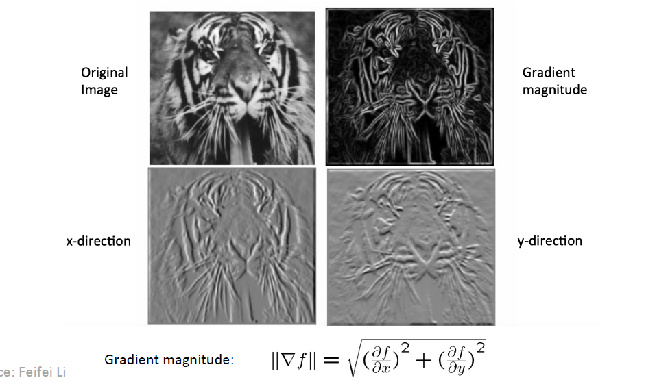
从这个意义上来说,我们可以求图片的 gradient \displaystyle \nabla f = \left[ \frac{\partial f}{\partial x}, \frac{\partial f}{\partial y}\right], in practice, use \displaystyle \frac{\partial f}{\partial x} |_{x = x_0} = \frac{f(x_0+1, y_0) - f(x_0-1, y_0)}{2}, 指定 gradient magnitude \displaystyle||\nabla f|| = \sqrt{(\frac{\partial f}{\partial x})^2 + (\frac{\partial f}{\partial y})^2}, 指向与edge垂直的方向
Filter
form a new image from original pixels, extract useful information. Modify properties
-
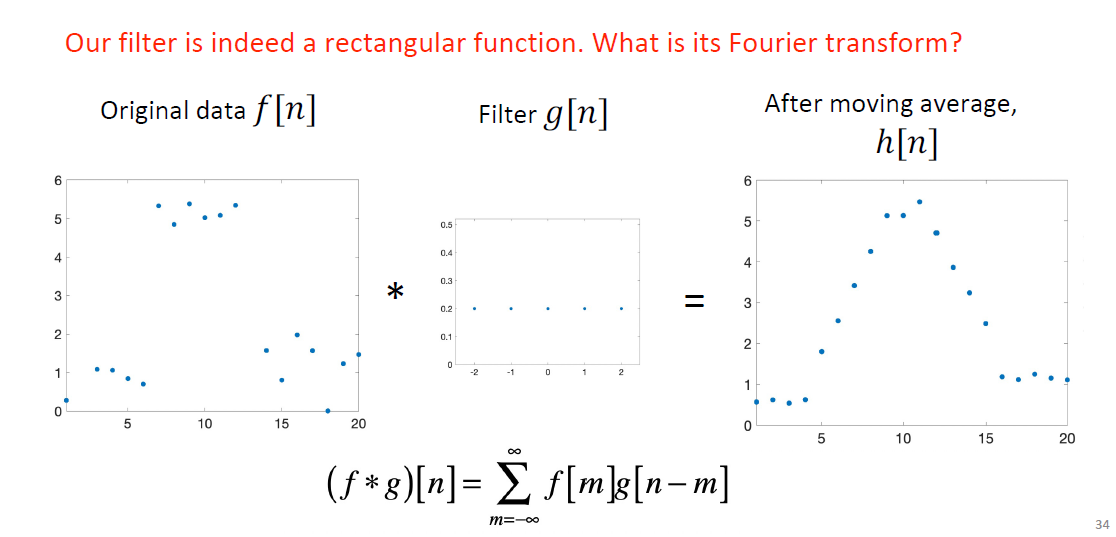
1D Filter: 线性, 噪声抑制 h = G(f), h[n] = G(f)[n], 一个例子是 \displaystyle h[n] = \frac{\sum_{i=-2}^{i=2} f(x+i)}{5}
-
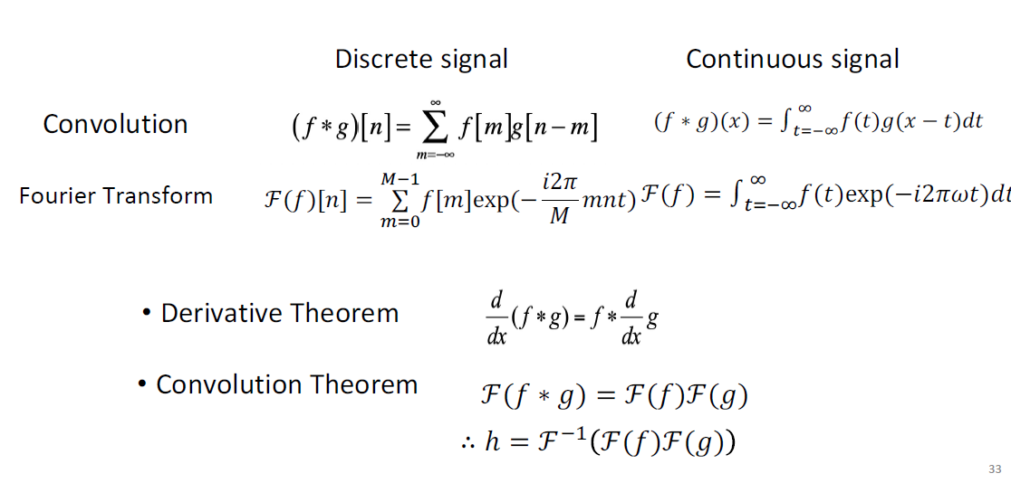
卷积 (convolution, 信号与系统) \displaystyle h[n] = (f*g)[n] = \sum_{m = -\infty}^{+\infty} f[m]g[n-m], 一个解释是 g 翻转再与 f 对位求积
-
最重要的卷积定理: For Fourier Transform F, F(f*g) = F(f)F(g), 时域的卷积等于频谱的乘积.
-
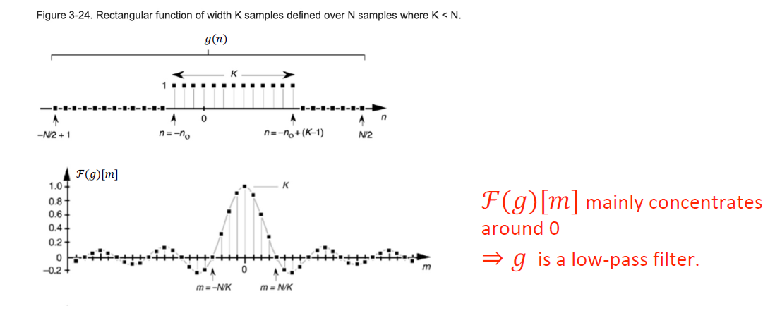
Fourier Transform gives F(g)[m] that mainly concentrates around 0, it's its main feature
g act as a 低通滤波器 low-pass filter
从 Convolution Theorem 解释就能发现卷积提取特征的原因: 滤去高频, 留下低频, 滤去噪声 =>
filtering G is linear. -
if says loss is 结果频率的纯性, 我们通过学习找到最好的g的weight
2D Discrete Filter
\displaystyle (f*g)[m, n] = \sum_{k, l} f[k, l]g[m-k, n-l], says g as kernal or filter
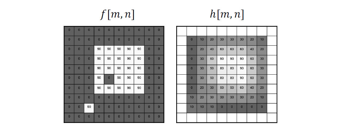
使用平均的 kernal 去除了 90 的高频信号但模糊了不是特别应该模糊的边界, 边界一定是高频的- 再进行一次二值化, 定义 threshold 阈值\tau, \displaystyle h[m, n] = \left\{ \begin{aligned} & 1, f[n, m] > \tau \\ & 0, \text{otherwise} \end{aligned} \right., non-linear system
Edge Detection
- Define edge: formulation (研究范式: Definition first, MathOP而不是DOP)
a region that has significant intensity change along one direction but low change in its orthogonal direction - Evaluate (评价标准 Evaluation matrix)
思考一下不好的情况
Example:Low precision's \displaystyle Precision = \frac{1}{3}, Recall = 1.
思考如何评定对齐: \displaystyle localization = \max_{distanceT\to P} < \varepsilon.
目标: good precision, good recall, low localization; - Smooth:
- Problem. Use derivative.
But 处处不平滑的 noises 可以很好的 hacking gradients => smoothing first.- Gaussian Filter as g to smooth noises: \displaystyle g = \frac{1}{\sqrt{2\pi \sigma^2}} \exp{- \frac{x^2}{2\sigma^2}}, the better is \displaystyle F(g) = \exp{-\frac{\sigma^2 \omega^2}{2}}.
- The bigger \sigma is, the sharper F(g) is. 那么它就是更强的low-pass filter.
- The smaller, the filter weaker.
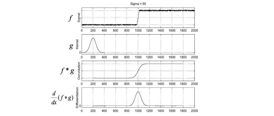
- Optimize: theorem \displaystyle \frac{d}{dx} (f*g) = f* \frac{d}{dx} g, 将两步合为一步
- 2D Convolution: Gaussian Filter \displaystyle g = \frac{1}{2\pi \sigma^2} \exp{-\frac{x^2+y^2}{2 \sigma^2}}. Use Optimize again.
- Binaryzation
结果: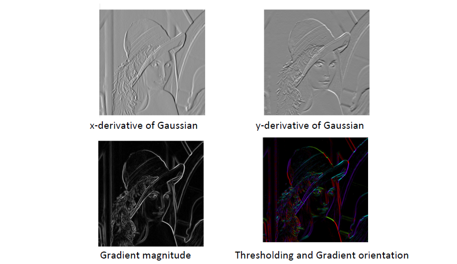
- Problem. Use derivative.
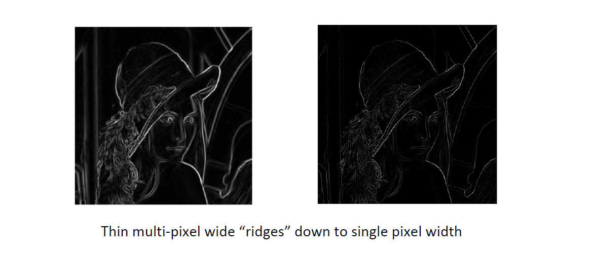
- NMS: 问题是存在宽度大于1的成分, 我们要去除 Non-Maximal 的成分, 只留下最好的
- Strategy
-
Get choice q and its gradient g(q)
-
Find neighbors (Another two choices): r = q + g(q), p = q - g(q).
Problem: r and p (大多时候)都是非格点, 没有函数值, 怎么办? 进行双线性插值 bilinear interpolation.
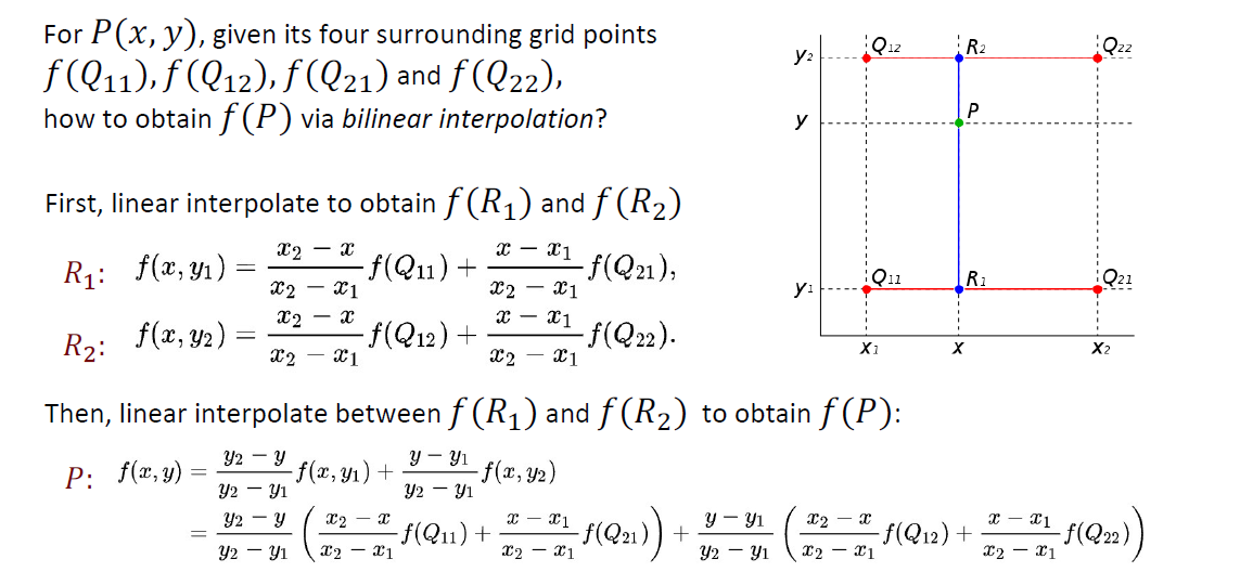
很好的是插值结果与投影方向无关. 对线性插值进行了性质很优的延拓.Another approach: 直接对齐到格点上, 性能很优.
-
Get g(p) and g(r).
-
g(p) < g(q) > g(r) proves q is a maxium.
-
- 结果
- Strategy
- Edge linking: Hysteresis Thresholding 滞回阈值(乱搞)
- gradient > maxVal => begin
- gradient < minVal => remove
- gradient between min and max => connect but no begin
Canny Edge Detector
Use:
- first derivative
- Gaussian kernal
- optimize signal-to-noise ratio to maxium precision & recall
超参\sigma:
- bigger \sigma, bigger precision
- smaller \sigma, smaller recall